Workflow Implementations in Python

MIAAIM’s workflows can also be run in Python to allow for more user flexibility with custom workflow creation. To install MIAAIM in Python, follow these steps:

Image Preparation (HDIprep)

The HDIprep workflow can be used in Python, just as it can be used in the command line interface. Commands are sequentially applied to images and are specified by the user.

Steady-state UMAP compression

Here, we will run through an example of using the HDIprep workflow in MIAAIM to create steady-state UMAP embeddings of a high-dimensional image data set. We will be using the mass spectrometry imaging data from prototype-001:

1. First import the necessary modules. We will also define a helper function to create plots after UMAP embedding.

# import hdi utils module
import hdiutils.HDIimport.hdi_reader as hdi_reader
# import hdi_prep module
from miaaim.hdiprep.HDIprep import hdi_prep
# import external modules
import matplotlib.pyplot as plt
from sklearn.preprocessing import minmax_scale
import matplotlib.patches as mpatches

# create function for easy plotting
def plot_rgb_2D(
                embedding,
                axs=(0,1),
                cols=(0,1,2),
                out_name=None
                ):
    """
    helper function for plotting 2D scatter plots from dimension reduction method.

    axs: tuple of 2 integers indicating which axes to extract for plotting
    cols: tuple of 3 integers indicating which axes to use for RGB coloring
    out_name: name to export image as (if None, then no image exported)
    """

    # create rgb scale based off first 3 channel
    rgb=minmax_scale(embedding[:,cols])
    # extract the columns to plot
    to_plot=embedding[:, axs]

    # create manual legend items for plotting purposes
    red_patch = mpatches.Patch(color='red', label='UMAP 1')
    green_patch = mpatches.Patch(color='green', label='UMAP 2')
    blue_patch = mpatches.Patch(color='blue', label='UMAP 3')

    # scatter plot
    fig, ax = plt.subplots()
    plt.scatter(to_plot[:,0],to_plot[:,1],color=rgb,s=15,linewidths=0)
    fig.suptitle('Steady State UMAP Embedding', fontsize=12)
    plt.xlabel('UMAP {}'.format(str(axs[0]+1)), fontsize=12)
    plt.ylabel('UMAP {}'.format(str(axs[1]+1)), fontsize=12)
    plt.legend(handles=[red_patch,green_patch,blue_patch],title='Linear Scale')
    plt.savefig(out_name,dpi=400,pad_inches = 0.1,bbox_inches='tight')
    plt.close()

2. Next, we will import the data and run the steady-state UMAP embedding on the prototype dataset.

# read data with HDIutils
mov_im = hdi_reader.HDIreader(
                    path_to_data=path_to_im,
                    path_to_markers=None,
                    flatten=True,
                    subsample=None,
                    mask=None,
                    save_mem=True
                    )
# create data set using HDIprep module
mov_dat = hdi_prep.IntraModalityDataset([mov_im])
# apply steady state UMAP embedding
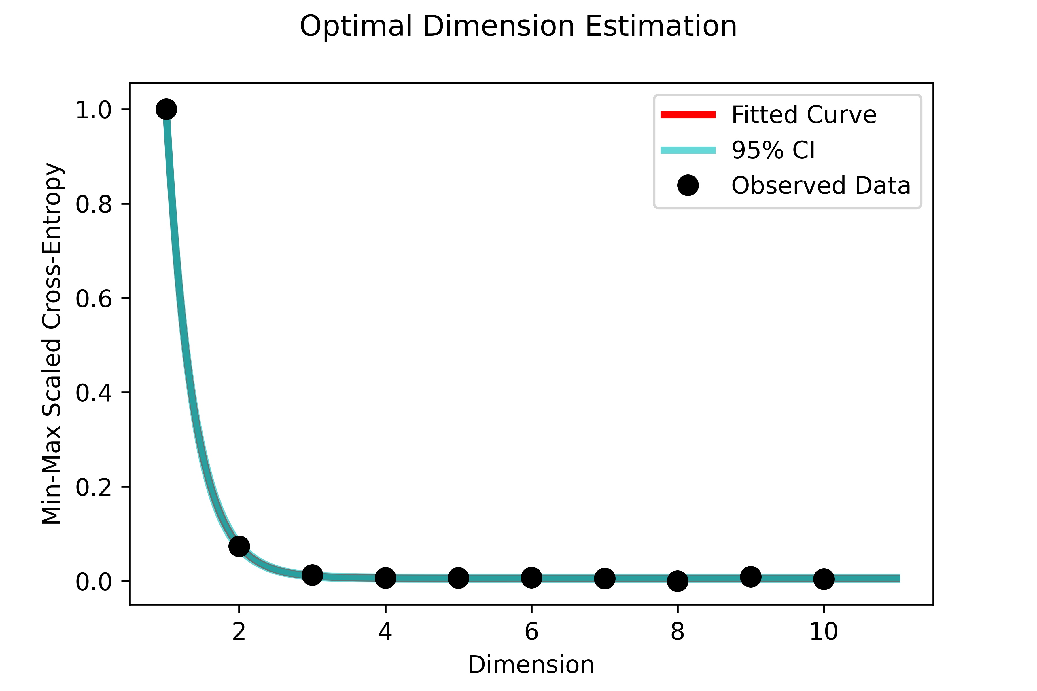
mov_dat.RunOptimalUMAP(
                        dim_range=(1,11),
                        landmarks=3000,
                        export_diagnostics=True,
                        output_dir=out_path,
                        n_jobs=1
                        )

Since we chose to export diagnostic plots using export_diagnostics=True, we obtained a resulting image of the exponential fit to the fuzzy set cross entropy that was used to compute the steady-state UMAP embedding:

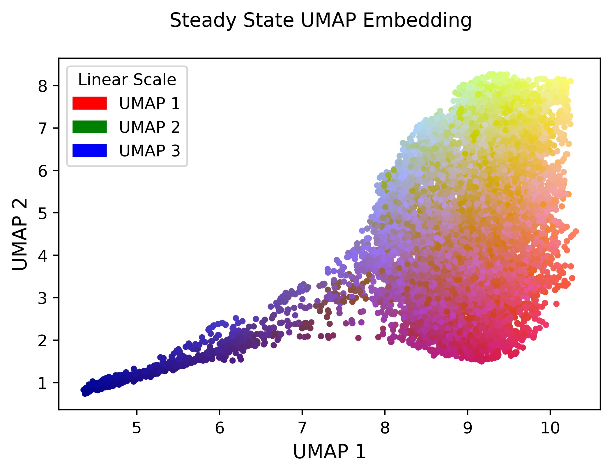
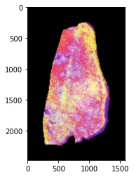
3. Now we can export a scatter plot of the 4-dimensional steady-state UMAP embedding in Euclidean space. Here the colors are RGB values created from the first 3 components of the embedding:

# for plotting purposes, extract the key of the umap embedding
key = list(mov_dat.umap_embeddings.keys())[0]
# plot the embedding of the UMAP in Euclidean space
embed = mov_dat.umap_embeddings[key]
# export a plot of the results in Euclidean space
plot_rgb_2D(embed.values, out_name="steady-state-UMAP-prototype-001.jpeg")

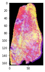
4. A final step to process prototype-001 is to reconstruct the original raster object using the coordinates of each pixel. Since the image was not a rectangular array, we will map it back to the spatial domain using the method="coordinate" option for the SpatiallyMapUMAP function.

Tip

Running steady-state image processing on data that is stored an array format follows the same process here, except the spatial mapping with SpatiallyMapUMAP uses the method="rectangular" option.

# reconstruct spatial image from UMAP embedding
mov_dat.SpatiallyMapUMAP(method="coordinate")
# extract processed image
proc_im = mov_dat.set_dict[key].hdi.data.processed_image
#plot the image using matplotlib (only the first 3 channels using RGB scale)
plt.imshow(proc_im[:,:,(0,1,2)])

5. The last step is to export the image for subsequent registration to its H&E stained counterpart. Here we export the image with padding and image resizing and view the results:

# export the processed image to the nifti format for image registration
# here we pad the image and resize it using bilinear interpolation for
# registration with the corresponding H&E image.
mov_dat.ExportNifti1(
                    output_dir="/Users/joshuahess/Desktop/",
                    padding="(20,20)",
                    target_size="(2472,1572)"
                    )
# load the exported image and view
exported = hdi_reader.HDIreader(
                    path_to_data="/Users/joshuahess/Desktop/prostate_processed.nii",
                    path_to_markers=None,
                    flatten=False,
                    subsample=None,
                    mask=None,
                    save_mem=False
                    )
# plot the exported image
plt.imshow(exported.hdi.data.image[:,:,(0,1,2)])

Histological Image Processing

Here we will demonstrate an example of running histology image processing on the H&E imaging modality. We will be using the prostate H&E imaging data from prototype-001 in the MIAAIM software.

1. First import the necessary modules.

# import hdi utils module
import hdiutils.HDIimport.hdi_reader as hdi_reader
# import hdi_prep module
from miaaim.hdiprep.HDIprep import hdi_prep
# import external modules
import matplotlib.pyplot as plt
import os

2. Now we will set the path to our imaging data and the output folders, and we will read in the imaging data set using the HDIreader class from the hdi-utils python package. We will then create a dataset using the HDIprep module imported above.

# set the path to the imaging data
path_to_im = "/Users/joshuahess/Desktop/prototype-001/input/fixed"
# set the path to the output directory
out_path = "/Users/joshuahess/Desktop/prototype-001/notebook-output"

# read data with HDIutils
fix_im = hdi_reader.HDIreader(
                 path_to_data=path_to_im,
                 path_to_markers=None,
                 flatten=False,
                 subsample=None,
                 mask=True,
                 save_mem=False
                 )
# create data set using HDIprep module
fix_dat = hdi_prep.IntraModalityDataset([fix_im])
# for plotting purposes, extract the key of the data set
key = list(fix_dat.set_dict.keys())[0]

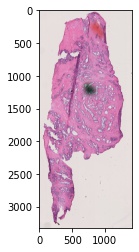
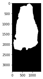
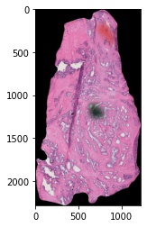
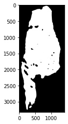
3. Now use the IntramodalityDataset class to run sequential morphological operations. Here we will show the input H&E image along with the manually drawn mask that we will use to help our image processing pipeline.

Note

All data are stored in the IntramodalityDataset as dictionary objects, kept under their filename as the key.

# plot the histology image
plt.imshow(fix_dat.set_dict[key].hdi.data.image)

# plot the input manually drawn mask in ImageJ
plt.imshow(fix_dat.set_dict[key].hdi.data.mask.toarray(),cmap='gray')

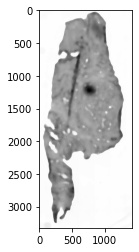
4. Next, we will convert the image to grayscale (carried out automatically in the MedianFilter function) and will use a median filter to remove salt and pepper noise in the image prior to the thresholding process.

# apply sequential processing steps
# remove salt and pepper noise
fix_dat.MedianFilter(filter_size=25,parallel=False)
# extract the procesed image to show
plt.imshow(fix_dat.set_dict[key].hdi.data.processed_image,cmap='gray')

5. After filtering, we will use the otsu automatic thresholding method to convert the grayscale image into a binary mask separating foreground from background.

# create mask with thresholding
fix_dat.Threshold(type='otsu')
# extract the procesed image to show
plt.imshow(fix_dat.set_dict[key].hdi.data.processed_image.toarray(),cmap='gray')

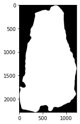
6. After thresholding, we will perform a series of morphological operations on the mask to smooth edges, fill holes, and connect regions in the mask that should represent the foreground (where the tissue is).

# morphological opening
fix_dat.Open(disk_size=20,parallel=False)
# extract the procesed image to show
plt.imshow(fix_dat.set_dict[key].hdi.data.processed_image.toarray(),cmap='gray')

# morphological closing
fix_dat.Close(disk_size=40,parallel=False)
# extract the procesed image to show
plt.imshow(fix_dat.set_dict[key].hdi.data.processed_image.toarray(),cmap='gray')

# morphological fill
fix_dat.Fill()
# extract the procesed image to show
plt.imshow(fix_dat.set_dict[key].hdi.data.processed_image.toarray(),cmap='gray')

# morphological opening
fix_dat.Open(disk_size=15,parallel=False)
# extract the processed image to show
plt.imshow(fix_dat.set_dict[key].hdi.data.processed_image.toarray(),cmap='gray')

# apply the manual input mask (will act on the previous masks)
fix_dat.ApplyManualMask()
# extract the processed image to show
plt.imshow(fix_dat.set_dict[key].hdi.data.processed_image.toarray(),cmap='gray')

# extract bounding box in the image for constant padding
fix_dat.NonzeroBox()
# extract the processed image to show
plt.imshow(fix_dat.set_dict[key].hdi.data.processed_image.toarray(),cmap='gray')

# apply the final mask after all operations
fix_dat.ApplyMask()
# extract the processed image to show
plt.imshow(fix_dat.set_dict[key].hdi.data.processed_image)

7. We will now add padding to the edges of the image to register this image to our mass spectrometry imaging data set. We recommend being a little generous with how much padding you add – leaving too little room on the edges of your image may make the registration optimization more difficult.

We will export the image with padding and read it back into our session to view the results:

# export the processed image to the nifti format for image registration
# here we pad the image for registration with the corresponding MSI
# compressed image.
fix_dat.ExportNifti1(
                    output_dir=out_path,
                    padding="(150,150)",
                    target_size=None
                    )

# load the exported image and view
exported = hdi_reader.HDIreader(
                    path_to_data=os.path.join(out_path,"fixed_processed.nii"),
                    path_to_markers=None,
                    flatten=False,
                    subsample=None,
                    mask=None,
                    save_mem=False
                    )
# plot the exported image
plt.imshow(exported.hdi.data.image)

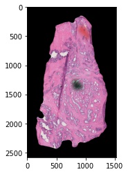
Image Registration (HDIreg)

The HDIreg workflow in Python is split into two modules, just as it is in Nextflow – the elastix and transformix workflows. Here, we will show both of them on the same data – prototype-001.

elastix

1. First import the necessary modules.

# import hdi utils module
import hdiutils.HDIimport.hdi_reader as hdi_reader
# import elastix and transformix modules
from miaaim.hdiprep.HDIprep import hdi_prep
from miaaim.hdireg.HDIreg import elastix
from miaaim.hdireg.HDIreg import transformix
# import external modules
import matplotlib.pyplot as plt
import os

2. Now we will set the path to our processed imaging data and the output folder, and we will read in the imaging data set using the HDIreader class from the hdi-utils python package. We will then create a dataset using the HDIprep module imported above. We will set the path to both the fixed image (the H&E modality) and a moving image (the steady-state UMAP compressed image).

Note

You do not need to import these modules to run elastix and transformix from the hdi-reg module. We are importing them so that we can easily plot the results of the registration process.

# set the path to the processed imaging data from hdiprep modules
path_to_fixed = r"D:\Josh_Hess\prototype-001\notebook-output\fixed_processed.nii"
path_to_moving = r"D:\Josh_Hess\prototype-001\notebook-output\moving_processed.nii"
# set the path to the output directory
out_dir = r"D:\Josh_Hess\prototype-001\notebook-output"

# read data with HDIutils
fix_im = hdi_reader.HDIreader(
                    path_to_data=path_to_fixed,
                    path_to_markers=None,
                    flatten=False,
                    subsample=None,
                    mask=False,
                    save_mem=False
                    )
# create data set using HDIprep module
fix_dat = hdi_prep.IntraModalityDataset([fix_im])
# for plotting purposes, extract the key of the data set
fix_key = list(fix_dat.set_dict.keys())[0]

# read data with HDIutils
mov_im = hdi_reader.HDIreader(
                    path_to_data=path_to_moving,
                    path_to_markers=None,
                    flatten=False,
                    subsample=None,
                    mask=False,
                    save_mem=False
                    )
# create data set using HDIprep module
mov_dat = hdi_prep.IntraModalityDataset([mov_im])
# for plotting purposes, extract the key of the data set
mov_key = list(mov_dat.set_dict.keys())[0]

# plot the histology image
plt.imshow(fix_dat.set_dict[fix_key].hdi.data.image)

# plot the moving steady state UMAP compressed image (note that we are only showing
# the first three channels in RGB space)
plt.imshow(mov_dat.set_dict[mov_key].hdi.data.image[:,:,:3])

3. Next, we will register these two images using the HDIreg workflow and the manifold alignment scheme. We will do this by first registering the images using an affine transformation, and then the images will be registered nonlinearly. These are indicated in the input folder of prototype-001 by the affine.txt and nonlinear.txt parameter files.

First, we set the paths to our parameter files and create a list from the two.

Note

Elastix uses file paths as input rather than any objects from the HDIprep module.

# set path to affine registration parameters
affine_pars = r"D:\Josh_Hess\prototype-001\input\affine_short.txt"
# set path to affine registration parameters
nonlinear_pars = r"D:\Josh_Hess\prototype-001\input\nonlinear_short.txt"
# concatenate the two parameter files to a list
p = [affine_pars, nonlinear_pars]

4. Now we can register the images using the elastix module.

Note

There are two pairs of elastix registration parameter files in the input folder for prototype-001. Here we use the shorter version for registration. The original version took ~1 hour to complete. The short version took ~40min using this dataset. If you are not using a machine with a lot of computing power, consider using the short version, as shown here. The short version was created by changing the number of resolutions and the number of spatial samples in the registration parameter files.

# run the registration
elastix.Elastix(path_to_fixed,
                path_to_moving,
                out_dir,
                p,
                fp=None,
                mp=None,
                fMask=None
                )

In the nonlinear parameter file, nonlinear.txt, we chose to export a r esulting image from elastix after registration using the WriteResultImage option. The output of this registration will be labelled with the suffix .1 since it is the second registration (the first registration would have exported an image with the .0 suffix).

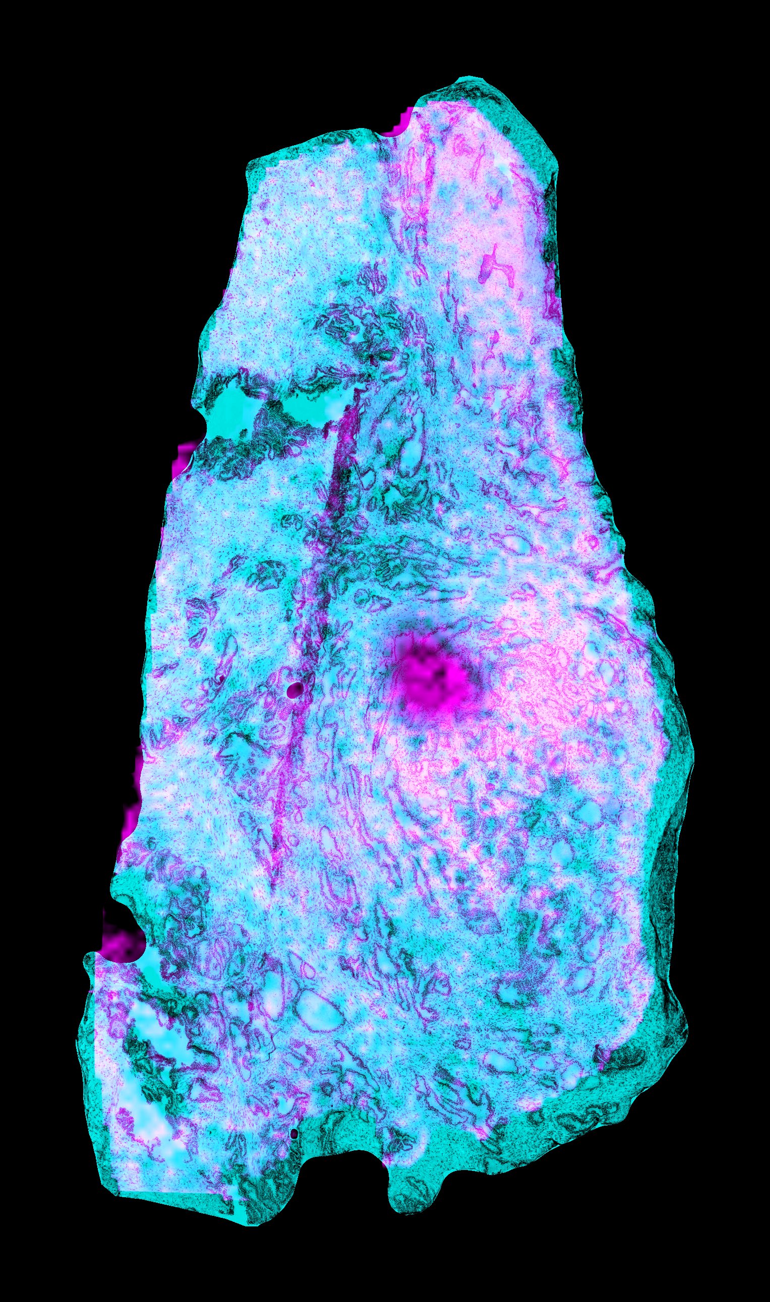
5. We can check the registration results by loading the images into ImageJ/FIJI. Here we exported an overlay of one of the H&E images and the resulting image from elastix. We saved the file as elastix-fiji-stack.tif. The cyan channel is the H&E modality, and the magenta channel is a channel from the MSI steady state compressed image.

Note

Elastix will only export the first channel if you using the WriteResultImage option. The full image stack can be exported using transformix, which we will show in a moment.

# set path to output image
result_path = r"D:\Josh_Hess\prototype-001\notebook-output\elastix-fiji-stack.tif"
# read the output image stack for registration results
result = hdi_reader.HDIreader(
                    path_to_data=result_path,
                    path_to_markers=None,
                    flatten=False,
                    subsample=None,
                    mask=False,
                    save_mem=False
                    )
# create data set using HDIprep module
result_dat = hdi_prep.IntraModalityDataset([result])
# for plotting purposes, extract the key of the data set
result_key = list(result_dat.set_dict.keys())[0]

# plot the histology image
plt.imshow(result_dat.set_dict[result_key].hdi.data.image)

transformix

6. Now, we can transform the original moving image using the elastix registration transform parameters. These are stored as TransformParameters.0.txt and TransformParameters.1.txt, again numbered according to the registration used (affine vs. nonlinear).

We set the path to the image registration parameters, the original moving image, and we set the pad width and target image size that were used during the HDIprep module (see notebook 001). All padding and image resizing is carried out on a per channel basis in Transformix.

Note

Note that running transformix on prototype-001 took ~8min on this machine, transformix 191 channels from the MSI data. The resulting file, moving_result.nii, is stored here as a .nii stack, and is ~5.86 GB.

# set path to moving image
in_im = r"D:\Josh_Hess\prototype-001\input\moving"
# set path to output transform parameter files
tps = [r"D:\Josh_Hess\prototype-001\notebook-output\TransformParameters.0.txt",
        r"D:\Josh_Hess\prototype-001\notebook-output\TransformParameters.1.txt"]
# set target size and padding (see notebook 001 for details)
target_size = (2472,1572)
pad = (20,20)

# transform the set of MSI data
transformix.Transformix(in_im,
                        out_dir,
                        tps,
                        target_size,
                        pad,
                        trim = None,
                        crops = None,
                        out_ext = ".nii"
                        )

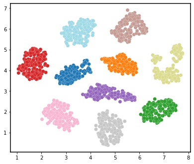
Tissue State Modeling (PatchMAP)

Here, we will show how to stitch together data by demonstrating cobordism learning in the PatchMAP workflow with the digits dataset.

1. First import the necessary modules.

# import patchmap module
from miaaim.patchmap import patchmap_
from miaaim.patchmap import utils
# import external modules
import scipy.sparse
from sklearn.datasets import load_digits
import matplotlib
import pandas as pd
import numpy as np
import matplotlib.pyplot as plt
import os

2. Now we will we will read in the example data from the digits dataset. We will then cut each individual digit into its own data frame to feed as input to the compute_cobordism function of the patchmap workflow.

# Load digits data
digits = load_digits()
dat = pd.DataFrame(digits['data'])
# Get the factor manifold IDs
nms = pd.DataFrame(digits['target'],columns=["target"])
# Create a combined data frame with names and data
dat_pd = pd.concat([dat,nms],axis=1)

# Create a list to store all digits in
digits_pd_list = []
digits_np_list = []
# Iterate through digits and create datafames for stitiching
for i in range(0,10):
    # Hold out digit i
    tmp = dat_pd.loc[dat_pd["target"]==i]
    # Update the pandas list
    digits_pd_list.append(tmp)
    # Update the numpy list
    digits_np_list.append(tmp.iloc[:,:64].values)

# Concatenate the lists
pandas_digits = pd.concat(digits_pd_list)
np_digits = np.vstack(digits_np_list)
# Create a colormap for the chosen labels
cmap = utils.discrete_cmap(len(pandas_digits['target'].unique()), 'tab20_r')
# Create colors
colors = [cmap(i) for i in pandas_digits['target']]

3. Now use the compute_cobordism function to create a higher-dimensional manifold that models similarity between each of the digits in the dataset.

# set number of nearest neighbors
nn = 150
# run the simiplicial set patching
patched_simplicial_set = patchmap_.compute_cobordism(
                                    digits_np_list,
                                    n_neighbors = nn
                                    )

4. Now embed the cobordism into two-dimensional space for visualization.

# embed the data
out = patchmap_.embed_cobordism(
                                digits_np_list,
                                patched_simplicial_set,
                                2,
                                n_epochs=200,
                                random_state=2,
                                min_dist = 0.1
                                )

# plot the results of embedded data
plt.rcParams['axes.linewidth'] = 1.5
fig, ax = plt.subplots(figsize=[6.5, 5.5])
im = ax.scatter(out[:,0], out[:,1], c = colors, s=50,cmap=cmap, edgecolor='white',linewidths=0.2)

Cross-System/Tissue Information Transfer (i-PatchMAP)